Scatterplots5
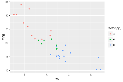
cinderplot
cinderplot 'data/mtcars.csv
  + aes(wt, mpg, colour=factor(cyl))
  + geom_point()' \
  -o out.svg
R
ggplot(mtcars, aes(wt, mpg, colour = factor(cyl))) + geom_point()
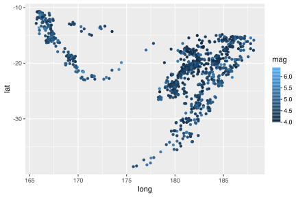
cinderplot
cinderplot 'data/quakes.csv
  + aes(long, lat, colour=mag)
  + geom_point()
  + scale_colour_gradient(low="#132b43", high="#56b1f7")' \
  -o out.svg
R
ggplot(quakes, aes(long, lat, colour = mag)) + geom_point() +
  scale_colour_gradient(low = "#132b43", high = "#56b1f7")
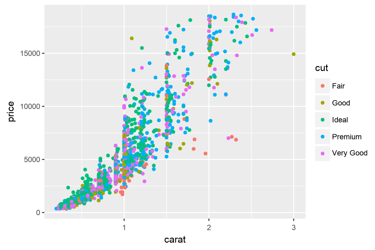
cinderplot
cinderplot 'data/diamonds_sample.csv
  + aes(carat, price, colour=cut)
  + geom_point()' \
  -o out.png
R
# diamonds, a 2000-row sample
ggplot(diamonds, aes(carat, price, colour = cut)) + geom_point()
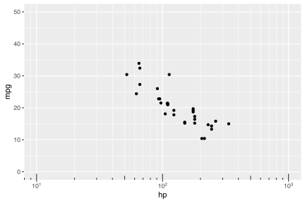
cinderplot
cinderplot 'data/mtcars.csv
  + aes(hp, mpg)
  + geom_point()
  + scale_x_log10(limits=c(10,1000))
  + ylim(0, 50)' \
  -o out.svg
R
ggplot(mtcars, aes(hp, mpg)) + geom_point() +
  scale_x_log10(breaks = trans_breaks("log10", function(x) 10^x),
                labels = trans_format("log10", math_format(10^.x)),
                limits = c(10, 1000)) +
  annotation_logticks(sides = "b") + ylim(0, 50)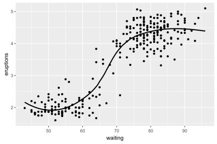
cinderplot
cinderplot 'data/faithful.csv
  + aes(waiting, eruptions)
  + geom_point()
  + geom_smooth(se=FALSE)' \
  -o out.svg
R
ggplot(faithful, aes(waiting, eruptions)) + geom_point() +
  geom_smooth(se = FALSE)
Annotations4
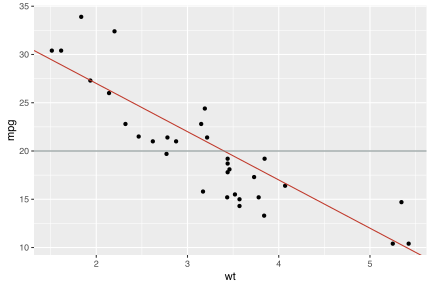
cinderplot
cinderplot 'data/mtcars.csv
  + aes(wt, mpg)
  + geom_point()
  + geom_abline(slope=-5, intercept=37, color="#c0392b")
  + geom_hline(yintercept=20, color="#7f8c8d")' \
  -o out.svg
R
ggplot(mtcars, aes(wt, mpg)) + geom_point() +
  geom_abline(slope = -5, intercept = 37, colour = "#c0392b") +
  geom_hline(yintercept = 20, colour = "#7f8c8d")
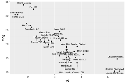
cinderplot
cinderplot 'data/mtcars.csv
  + aes(wt, mpg, label=model)
  + geom_point()
  + geom_text_repel(size=2.6)' \
  -o out.svg
R
# mtcars model names, ggrepel-style placement
library(ggrepel)
ggplot(mtcars, aes(wt, mpg, label = rownames(mtcars))) +
  geom_point() + geom_text_repel(size = 2.6)
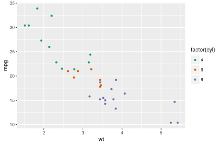
cinderplot
cinderplot 'data/mtcars.csv
  + aes(wt, mpg, colour=factor(cyl))
  + geom_point()
  + scale_colour_manual(values=c("4"="#1b9e77","6"="#d95f02","8"="#7570b3"))' \
-o out.svgR
ggplot(mtcars, aes(wt, mpg, colour = factor(cyl))) + geom_point() +
  scale_colour_manual(values = c("4"="#1b9e77","6"="#d95f02","8"="#7570b3"))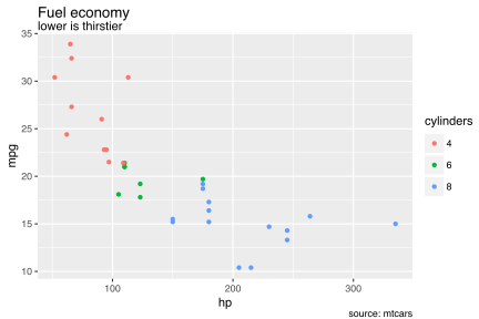
cinderplot
cinderplot 'data/mtcars.csv
  + aes(hp, mpg, colour=factor(cyl))
  + geom_point()
  + labs(title="Fuel economy", subtitle="lower is thirstier", caption="source: mtcars", colour="cylinders")' \
  -o out.svg
R
ggplot(mtcars, aes(hp, mpg, colour = factor(cyl))) + geom_point() +
  labs(title = "Fuel economy", subtitle = "lower is thirstier",
caption = "source: mtcars", colour = "cylinders")Distributions2
cinderplot
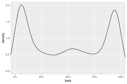
cinderplot 'data/gm12878_betas.tsv
  + aes(beta)
  + geom_density()
  + scale_x_continuous(labels=percent)' \
  -o out.svg
R
# GM12878 methylation betas (bimodal)
ggplot(betas, aes(beta)) + geom_density() +
  scale_x_continuous(labels = scales::percent)
cinderplot
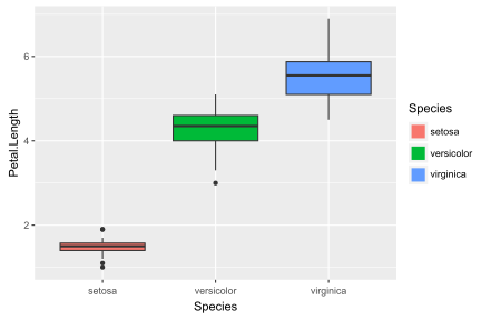
cinderplot 'data/iris.csv
  + aes(x=Species, y=Petal.Length, fill=Species)
  + geom_boxplot()' \
  -o out.svg
R
ggplot(iris, aes(Species, Petal.Length, fill = Species)) + geom_boxplot()
Small multiples1
cinderplot
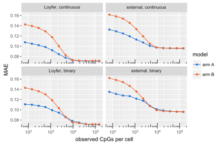
cinderplot 'data/upscale_mae.csv
  + aes(coverage, mae, colour=model)
  + geom_line()
  + geom_point()
  + facet_wrap(~panel, levels=c("Loyfer, continuous", "external, continuous", "Loyfer, binary", "external, binary"))
  + scale_x_log10()
  + scale_colour_manual(values=c("#2a78d6","#eb6834"))
  + labs(x="observed CpGs per cell", y="MAE")' \
-o out.svgR
# panel order is set by the factor levels, not alphabetical
ggplot(transform(upscale, panel = factor(panel,
         levels = c("Loyfer, continuous", "external, continuous",
                    "Loyfer, binary", "external, binary"))),
       aes(coverage, mae, colour = model)) +
  geom_line() + geom_point() + facet_wrap(~panel) +
  scale_x_log10() +
  scale_colour_manual(values = c("#2a78d6", "#eb6834")) +
labs(x = "observed CpGs per cell", y = "MAE")Heatmaps1
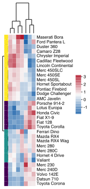
cinderplot
cinderplot 'data/mtcars_heat.csv
  + heatmap(name="m", cluster=both, rownames=right)
  + dendrogram(top_of("m"))
  + annotation("data/mtcars_cyl.csv", left_of("m"), name="cyl")
  + dendrogram(left_of("cyl"))
  + legend(right_of("m"))
  + scale_fill_gradient2(low="#2166ac", mid="#f7f7f7", high="#b2182b")' \
-o out.svgR
# mtcars, z-scored features (ComplexHeatmap)
library(ComplexHeatmap)
m <- scale(as.matrix(mtcars[, c("mpg","disp","hp","drat","wt","qsec","carb")]))
Heatmap(m, name = "z", cluster_rows = TRUE, cluster_columns = TRUE,
left_annotation = rowAnnotation(cyl = factor(mtcars$cyl)))Genomics4
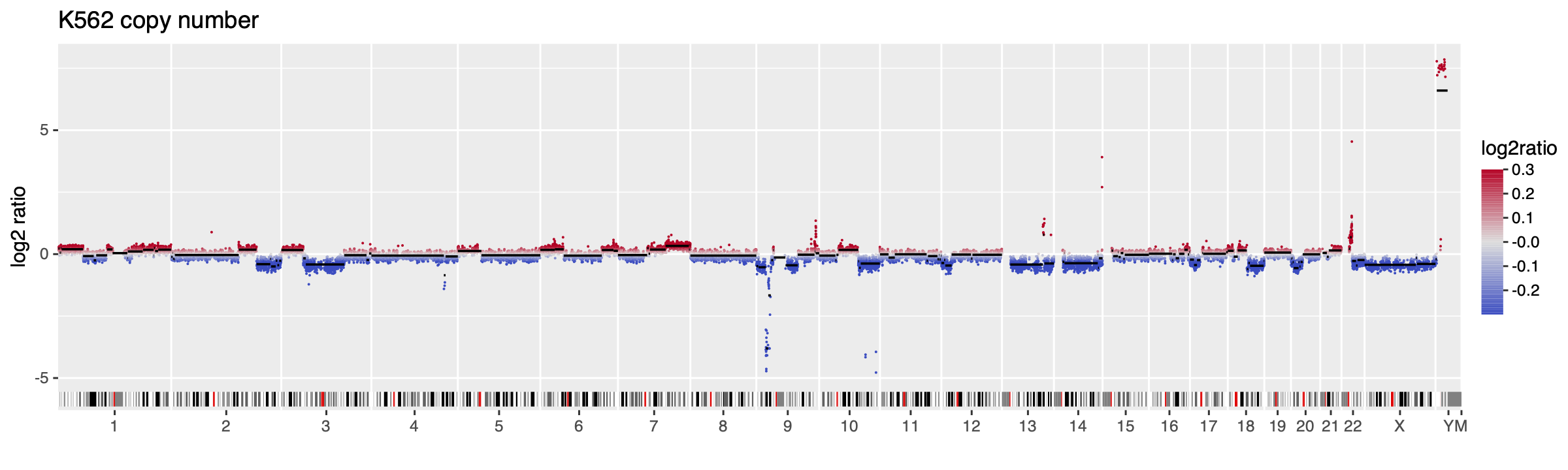
cinderplot
cinderplot 'data/k562.bins.tsv
  + aes(chrom=chrom, x=start, xend=end, y=log2ratio, colour=log2ratio)
  + geom_point(size=0.5)
  + geom_segment(data="data/k562.segments.tsv", y=seg.mean, color="black")
  + scale_x_genome("hg38/seqinfo.tsv.gz")
  + scale_colour_gradient2(low="#3b4cc0", mid="#dcdcdc", high="#b40426", midpoint=0, limits=c(-0.3,0.3))
  + ideogram("hg38/cytoband.tsv.gz")
  + labs(title="K562 copy number", y="log2 ratio")' \
-o out.png --size 12x3.6R
# K562 copy number, EPICv2 (sesame)
library(sesame)
visualizeSegments(cnv)  # bins + CBS segments + ideogram, whole-genome x
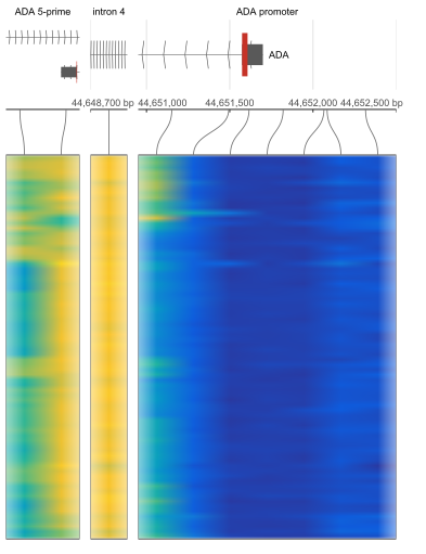
cinderplot
cinderplot 'regions("data/ada_windows.bed")
  + genes("hg38/genes.bed.gz", height=1.4)
  + matrix("data/region_betas_long.tsv", name="betas", cluster=samples, rownames=off, colnames=off, height=9)' \
-o out.svgR
# Gviz draws one region per plotTracks() call, so several loci means
# several figures stitched together outside R -- losing the shared
# sample order, the common colour scale and the single axis.
library(Gviz)
for (w in windows) plotTracks(tracks, chromosome = w$chr,
                              from = w$start, to = w$end)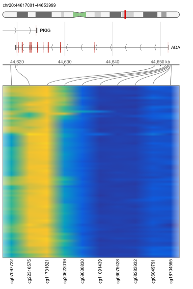
cinderplot
cinderplot 'region()
  + cytoband("hg38/cytoband.tsv.gz", height=0.5)
  + genes("hg38/genes.bed.gz", height=1.5)
  + matrix("data/region_betas_long.tsv", name="betas", cluster=samples, rownames=off, height=10)' \
-o out.svgR
# ADA locus methylation, HM450 (sesame)
library(sesame)
visualizeRegion("chr20", 44616522, 44655233, betas,
                platform = "HM450", cluster.samples = TRUE)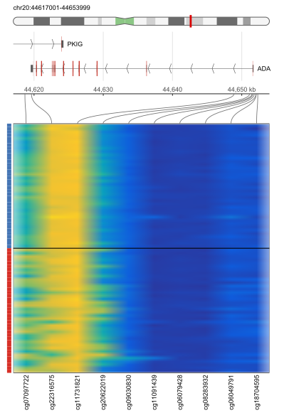
cinderplot
cinderplot 'region()
  + cytoband("hg38/cytoband.tsv.gz", height=0.5)
  + genes("hg38/genes.bed.gz", height=1.5)
  + matrix("data/region_betas_grouped.tsv", name="betas", cluster=none, rownames=off, rowmeta="data/region_betas_samples.tsv", rowbar="condition", rowcolour="data/region_betas_rowcol.tsv", height=10)' \
-o out.svgR
# Rows grouped by a sample-metadata column and labelled with a coloured
# band -- Gviz/ComplexHeatmap need separate annotation objects wired by
# hand; here it is one matrix() with rowmeta=/rowbar=.
Trees1
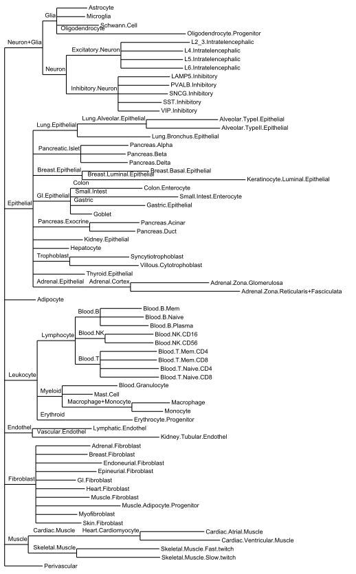
cinderplot
cinderplot 'data/celltype68.tre
  + geom_tree()
  + geom_tiplab()
  + geom_nodelab()' \
  -o out.svg
R
# 68 cell types, four levels; internal nodes carry the level names
library(ggtree)   # Bioconductor, and it needs ape for the parse
tr <- ape::read.tree("celltype68.tre")
ggtree(tr) + geom_tiplab() + geom_nodelab()Polar & chord2
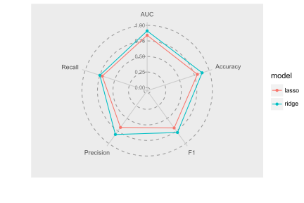
cinderplot
cinderplot 'data/radar_metrics.csv
  + aes(x=factor(metric), y=score, colour=model)
  + geom_line()
  + geom_point()
  + coord_polar()
  + ylim(0,1)' \
  -o out.svg
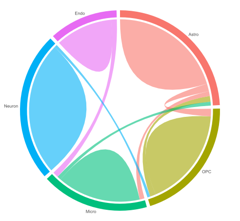
cinderplot
cinderplot 'data/chord_flows.csv
  + chord()' \
  -o out.svg
Colour palettes12
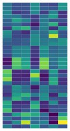
cinderplot
cinderplot 'data/mtcars_heat.csv
  + heatmap(name="m", cluster=none, rownames=none)
  + scale_fill_viridis()' \
  -o out.svg
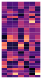
cinderplot
cinderplot 'data/mtcars_heat.csv
  + heatmap(name="m", cluster=none, rownames=none)
  + scale_fill_magma()' \
  -o out.svg
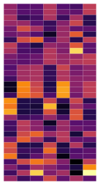
cinderplot
cinderplot 'data/mtcars_heat.csv
  + heatmap(name="m", cluster=none, rownames=none)
  + scale_fill_inferno()' \
  -o out.svg
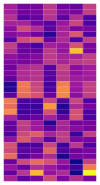
cinderplot
cinderplot 'data/mtcars_heat.csv
  + heatmap(name="m", cluster=none, rownames=none)
  + scale_fill_plasma()' \
  -o out.svg
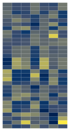
cinderplot
cinderplot 'data/mtcars_heat.csv
  + heatmap(name="m", cluster=none, rownames=none)
  + scale_fill_cividis()' \
  -o out.svg
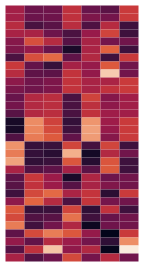
cinderplot
cinderplot 'data/mtcars_heat.csv
  + heatmap(name="m", cluster=none, rownames=none)
  + scale_fill_rocket()' \
  -o out.svg
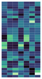
cinderplot
cinderplot 'data/mtcars_heat.csv
  + heatmap(name="m", cluster=none, rownames=none)
  + scale_fill_mako()' \
  -o out.svg
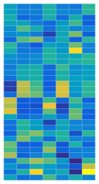
cinderplot
cinderplot 'data/mtcars_heat.csv
  + heatmap(name="m", cluster=none, rownames=none)
  + scale_fill_parula()' \
  -o out.svg
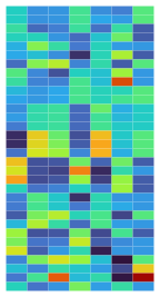
cinderplot
cinderplot 'data/mtcars_heat.csv
  + heatmap(name="m", cluster=none, rownames=none)
  + scale_fill_turbo()' \
  -o out.svg
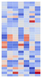
cinderplot
cinderplot 'data/mtcars_heat.csv
  + heatmap(name="m", cluster=none, rownames=none)
  + scale_fill_coolwarm()' \
  -o out.svg
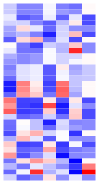
cinderplot
cinderplot 'data/mtcars_heat.csv
  + heatmap(name="m", cluster=none, rownames=none)
  + scale_fill_bwr()' \
  -o out.svg
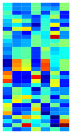
cinderplot
cinderplot 'data/mtcars_heat.csv
  + heatmap(name="m", cluster=none, rownames=none)
  + scale_fill_jet()' \
  -o out.svg
Themes8
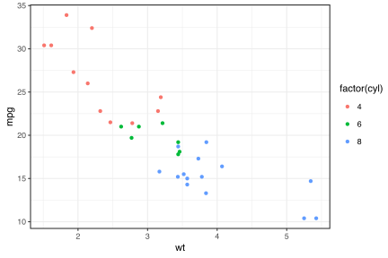
cinderplot
cinderplot 'data/mtcars.csv
  + aes(wt, mpg, colour=factor(cyl))
  + geom_point()
  + theme_bw()' \
  -o out.svg
R
ggplot(mtcars, aes(wt, mpg, colour = factor(cyl))) + geom_point() + theme_bw()
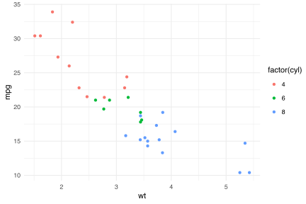
cinderplot
cinderplot 'data/mtcars.csv
  + aes(wt, mpg, colour=factor(cyl))
  + geom_point()
  + theme_minimal()' \
  -o out.svg
R
ggplot(mtcars, aes(wt, mpg, colour = factor(cyl))) + geom_point() + theme_minimal()
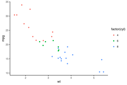
cinderplot
cinderplot 'data/mtcars.csv
  + aes(wt, mpg, colour=factor(cyl))
  + geom_point()
  + theme_classic()' \
  -o out.svg
R
ggplot(mtcars, aes(wt, mpg, colour = factor(cyl))) + geom_point() + theme_classic()
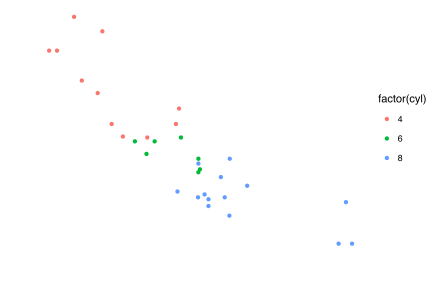
cinderplot
cinderplot 'data/mtcars.csv
  + aes(wt, mpg, colour=factor(cyl))
  + geom_point()
  + theme_void()' \
  -o out.svg
R
ggplot(mtcars, aes(wt, mpg, colour = factor(cyl))) + geom_point() + theme_void()
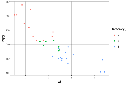
cinderplot
cinderplot 'data/mtcars.csv
  + aes(wt, mpg, colour=factor(cyl))
  + geom_point()
  + theme_linedraw()' \
  -o out.svg
R
ggplot(mtcars, aes(wt, mpg, colour = factor(cyl))) + geom_point() + theme_linedraw()
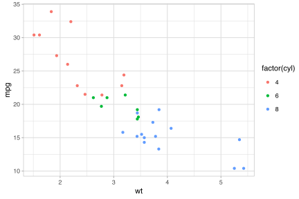
cinderplot
cinderplot 'data/mtcars.csv
  + aes(wt, mpg, colour=factor(cyl))
  + geom_point()
  + theme_light()' \
  -o out.svg
R
ggplot(mtcars, aes(wt, mpg, colour = factor(cyl))) + geom_point() + theme_light()
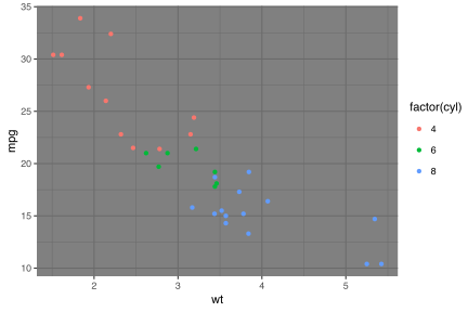
cinderplot
cinderplot 'data/mtcars.csv
  + aes(wt, mpg, colour=factor(cyl))
  + geom_point()
  + theme_dark()' \
  -o out.svg
R
ggplot(mtcars, aes(wt, mpg, colour = factor(cyl))) + geom_point() + theme_dark()
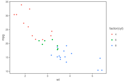
cinderplot
cinderplot 'data/mtcars.csv
  + aes(wt, mpg, colour=factor(cyl))
  + geom_point()
  + theme_few()' \
  -o out.svg
R
# requires ggthemes
ggplot(mtcars, aes(wt, mpg, colour = factor(cyl))) + geom_point() + theme_few()
Datasets used in these examples (mtcars, quakes, diamonds, …) are available from the cinderplot-examples repository.